CuTe Layout and Tensor

Disclaimer: The content of this blog reflects my personal experiences and opinions while learning GPU programming in my own time. All information presented is publicly available and does not represent the views or positions of NVIDIA Corporation or any of its affiliates.

0. Introduction

In this blog, I will introduce my understanding/interpretation of CuTe layout and tensor. It assumes some basic understanding of CuTe layout and tensor. You can refer to the additional references in Sec. 8 for the basic introduction of CuTe layout and tensor. The demo code of the operations mentioned in this blog can be found here.

A CuTe layout is a mapping from tensor coordinate to physical index/address in memory. A CuTe layout consists of 2 parts: Shape and Stride. Dimension is called mode in CuTe. Number of dimensions is called rank.

1. Shape and Stride

Shape is the shape of the tensor in the coordinate space. Shape<I> means the number of elements in the I-th dimension. Stride<I> at dimension I means if I increment the coordinate from i to i + 1, how much I need to increment the physical index in memory.

Default stride is LayoutLeft i.e. column major, this means stride[0] = 1, and subsequet stride is the prefix product of the shape from left to right. LayoutRight, i.e. row major, means stride[-1] = 1, and stride is the prefix product of the shape from right to left.

Shape : (M, N, K)
# LayoutLeft, column major
  Stride: (1, M, M * N)
# LayoutRight, row major
  Stride: (N * K, K, 1)

The shorthand representation of a layout is Shape : Stride, e.g. (M, N, K) : (1, M, M * N) is a column major layout.

1.1 Example Layout

A is the logical tensor view with (natural) coordinates in the coordinate space, storage is the physical 1D memory layout

# This describes a 4x2 row major matrix
Shape :  (4, 2)
Stride:  (2, 1)
m = [0, 4)
n = [0, 2)
A(m, n) # natural coordinate of tensor
  = storage[m * 2 + n * 1] # physical index in memory

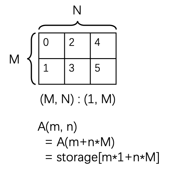
# Symbolically, this describes a MxN column major matrix
Shape:  (M, N)
Stride: (1, M)
m = [0, M)
n = [0, N)
A(m, n) # natural coordinate of tensor
  = storage[m * 1 + n * M] # physical index in memory

# This can still represent a 4x2 matrix
Shape:  ((2, 2), 2)
Stride: ((4, 1), 2)
m = [0, 2)
n = [0, 2)
k = [0, 2)
A((m, n), k) # natural coordinate of tensor
  = storage[m * 4 + n * 1 + k * 2] # physical index in memory

Natural coordinate has the same coordinate space as shape. this means if the shape is (M, N, K), then we have 3 natural coordinates, (m, n, k). If the shape is (M, (N, K, L)), then we have 4 natural coordinates, (m, (n, k, l)).

2. Coordinate Conversion

Natural coordinate is not the only way to index into a tensor. Equivalently, we can use 1D coordinate to index into a tensor. The conversion from natural coordinate to 1D coordinate is done by assigning a LayoutLeft to the natural coordinate shape.

Shape : (M, N, K)
Natural Coordinate Stride: (1, M, M * N)
Natural Coordinate: (m, n, k)
 = 1D Coordinate: (m + n * M + k * M * N)

Then you can access the tensor by using either the natural coordinate or the 1D coordinate.

# This describes a row major matrix
Shape :  (4, 2)
Stride:  (2, 1)
m = [0, 4)
n = [0, 2)
A(m, n) # natural coordinate of tensor
  = A (m + n * 4) # 1D coordinate of tensor
  = storage[m * 2 + n * 1] # physical index in memory

Knowing that, every CuTe layout can be viewed in 2 equivalent ways:

1. A mapping between natural coordinates (Int, Int, Int, …) to physical index (Int) in memory.
2. A mapping between 1d coordinate (Int) to physical index (Int) in memory. We call the 1d coordinate domain, and the physical index co-domain.

2.1 Size and Cosize

Size is just the number of elements in the domain (i.e. 1d coordinate). Cosize is the number of elements in the co-domain (i.e. physical index).

You can also get the Shape, Stride, Size, Cosize of a specific dimension (i.e. dimension I) of a layout by using shape<I>, stride<I>, size<I>, cosize<I> function.

Note that the difference between Size and Shape is that a Shape can be a tuple (multi-dimensional), but Size is a single integer counting the number of elements in the multi-dimensional shape.

3. Coalesce (a.k.a. dimension flattening)

In certain cases, a 2d layout is equivalent to a 1d layout. In the sense that every layout is Int->Int, the 2d layout has the same int to int mapping as the 1d layout.

One example would be (M, N) : (1: M) is equivalent to M * N : 1. Below is the proof:

# 2d layout
Shape : (M, N)
Stride: (1, M)
m = [0, M)
n = [0, N)
A(m, n) 
  = A(m + n * M)
  = storage[m + n * M]

# 1d layout
# substitute k = m + n * M
Shape : (M * N)
Stride: (1)
k = [0, M * N)
A(k)
  = A(k)
  = storage[k]

So if we have a layout (M, N) : (1, M), we can coalesce (a.k.a. dimension flattening) it to M * N : 1 by replacing the 2d coordinate (m, n) with k = m + n * M. Note that M * N : 1 is just a 1d identity mapping between natural coordinate (Int) and physical index (Int) in memory.

According to CuTe document, there are 3 cases where we can coalesce:

1. (s0, _1) : (d0, d1) => s0:d0. Ignore modes with size static-1.
2. (_1, s1) : (d0, d1) => s1:d1. Ignore modes with size static-1.
3. (s0, s1) : (d0, s0 * d0) => s0 * s1 : d0. If the second mode’s stride is the product of the first mode’s size and stride, then they can be combined.

3.1 By-mode coalesce

Sometimes, you just want to coalesce a sub-layout of a layout. In this case, you should use by-mode coalesce to preserve the original (higher level) shape of the layout.

For instance, if we have a layout ((M, N), K, L) : ((1, M), M * N, M * N * K), and we want to coalesce the sub-layout (M, N) : (1, M), we should use by-mode coalesce to preserve the original 3d shape of the layout. In code what we do is coalesce(layout, Step<_1, _1, _1>{});. Step<_1, _1, _1> here means we want the resulting layout to have rank 3, because Step<_1, _1, _1> has rank 3. CuTe will apply coalesce to each mode separately. The value inside Step<> doesn’t matter, only the rank of the Step<> matters. Then the result is (M * N, K, L) : (1, M * N, M * N * K).

4. Blocked Product

Sometimes we want a quite complex layout, an example of that is shown below:

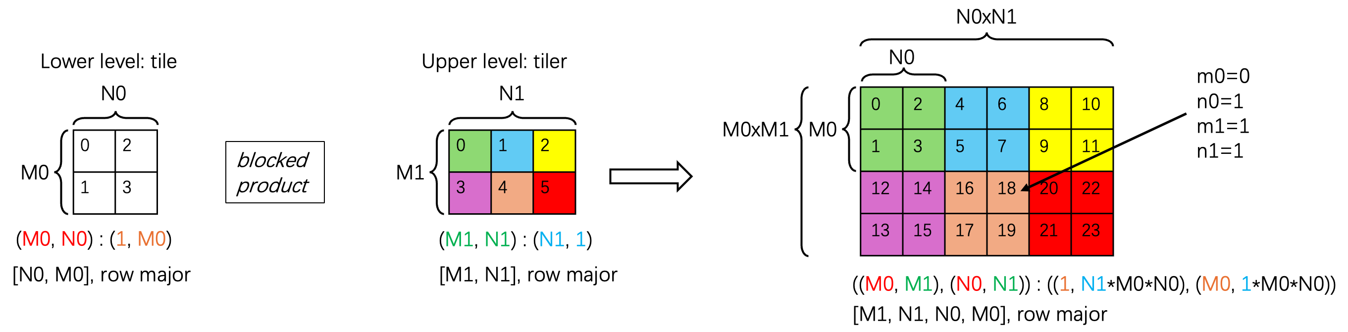
We have a 2d tile (M0, N0) : (1, M0) and we want to repeat it first along the N dimension N1 times and then along the M dimension M1 times to get the whole tensor on the right. And we call the layout that describes this repeat the tiler layout ((M1, N1) : (N1, 1)). As you can see from the layout, this tiler is row major, which means we repeat the tile along the N dimension first and then along the M dimension.

This operation is formally called blocked product in CuTe. The final “stacked” layout is:

2d tile layout: (M0, N0) : (1, M0)
tiler layout: (M1, N1) : (N1, 1)
blocked_product(2d tile, tiler)
 = (M0, N0) : (1, M0) * (M1, N1) : (N1, 1)
 = ((M0, M1), (N0, N1)) : ((1, N1*M0*N0), (M0, 1*M0*N0))

It’s kind of intuitive to see why this is the case. Intuitively this is a 4d tensor with shape [M1, N1, N0, M0], row major (by doing the blocked product of [N0, M0], row major with [M1, N1], row major). But we still want to keep the illusion that this is a 2d tensor that can be indexed by (m, n) coordinate. So we rearrange the shape of the final layout to ((M0, M1), (N0, N1)).

Next I will describe how we arrive at the stride of the final layout. The inner tile of (M0, N0) will just have stride 1 at M0 dimension and stride M0 at N0 dimension, the same as the original tile layout before stacking. Then what happens to the layout of dimension M1 and N1? Their strides simply get inflated by the size of the tile. We can focus on the top left element of the tile (value 0, 4, 8, 12, 16, 20 in the figure). Think about the N1 dimension, before it was 1, now with the tile repeat at a interval/size of N0, the interval between two consecutive coordinates in the N1 dimension is N0. The stride for M1 dimension is a little different, because we have to repeat the M0 * N0 tile at the N dimension N1 times first, then arrive at a new M1. So the interval between two consecutive coordinates in the M1 dimension is N1 * N0 * M0. In this way we calculate the stride of the final layout.

More concretely what this final layout describes is:

Shape : ((M0, M1), (N0, N1))
Stride: ((1, N1*M0*N0), (M0, 1*M0*N0))
m0 = [0, M0)
m1 = [0, M1)
n0 = [0, N0)
n1 = [0, N1)
A((m0, m1), (n0, n1)) # natural/4d coordinate of tensor
  = A(m0+m1*M0, n0+n1*N0) # 2d coordinate of tensor
  = storage[m0*1+m1*N1*M0*N0+n0*M0+n1*M0*N0] # physical index in memory

So you can kinda view it as a 4d tensor with index (m0, m1, n0, n1). But you can also view it as a 2d tensor (as shown in the figure) with index (m, n), where m is the 1d coordinate along the M dimension and n is the 1d coordinate along the N dimension.

The example element pointed by the arrow in the figure is:

M0 = 2, M1 = 2, N0 = 2, N1 = 3
m0 = 0, m1 = 1, n0 = 1, n1 = 1
A((m0, m1), (n0, n1)) = A((0, 1), (1, 1)) # natural/4d coordinate of tensor
  = A(m0+m1*M0, n0+n1*N0) = A(2, 3) # 2d coordinate of tensor
  = storage[m0*1+m1*N1*M0*N0+n0*M0+n1*M0*N0] = storage[18] # physical index in memory

There is one final piece of the story, above is not the most succinct way to describe the final layout, i.e. the N dimension can be further coalesced. It’s better explained by the following equation:

Shape : ((M0, M1), N0 * N1)
Stride: ((1, N1*M0*N0), M0)
m0 = [0, M0)
m1 = [0, M1)
n0 = [0, N0)
n1 = [0, N1)
# do the following substitution
n = [0, N0 * N1)
n = n0 + n1 * N0

A((m0, m1), (n0, n1)) # natural/4d coordinate of tensor
  = A((m0, m1), n) # substitute with n
  = A(m0+m1*M0, n0+n1*N0) # 2d coordinate of tensor
  = A(m0+m1*M0, n) # substitute with n
  = storage[m0*1+m1*N1*M0*N0+n0*M0+n1*M0*N0] # physical index in memory
  = storage[m0*1+m1*N1*M0*N0+n*M0] # substitute with n

So the final coalesced layout is ((M0, M1), N0 * N1) : ((1, N1*M0*N0), M0). Another way to represent this tensor is a 3d tensor with shape [M1, N0 * N1, M0], row major.

4.1 Logical Product

Logical product is the primitive blocked product calls when constructing the blocked product layout. You can think of the 1d logical product as the blocked product example above but with 1d tile and tiler. This means I just want to repeat the tile along the N dimension N1 times in my 1d logical product.

In theory, the blocked product we show above is just two 1d logical product that applied to M and N dimension separately. Because we just want to repeat N0 N1 times along the N dimension and M0 M1 times along the M dimension. But there are nuances to it. As we see above, to get the stride of M1, we actually need to know the size of N0 and N1, which means we can’t do two logical product on the two dimensions separately and stitch them together. Logical product in M dimension needs information from N dimension and vice versa.

So here comes the blocked product which is a special form of 2 1d logical product that takes into account the stride dependency between M and N dimension. More specifically, it takes the M dimension logical product first and then use the result to do the N dimension logical product.

5. Local Tile (a.k.a. Inner Partitioning/Slicing)

Often times, we want to tile/partition a tensor into smaller sub-tiles and each sub-tile is processed by a parallel agent (e.g. CTA). The most common way form of tiling is to use the local_tile function (inner_partition is the official/equivalent CuTe layout algebra function).

Suppose we want to re-partition the final layout (in the blocked product example above) ((M0, M1), (N0, N1)) : ((1, N1*M0*N0), (M0, 1*M0*N0)) into many 2d sub-tiles, with each sub-tile of shape (M0, N0). The figure below shows this partitioning scheme.

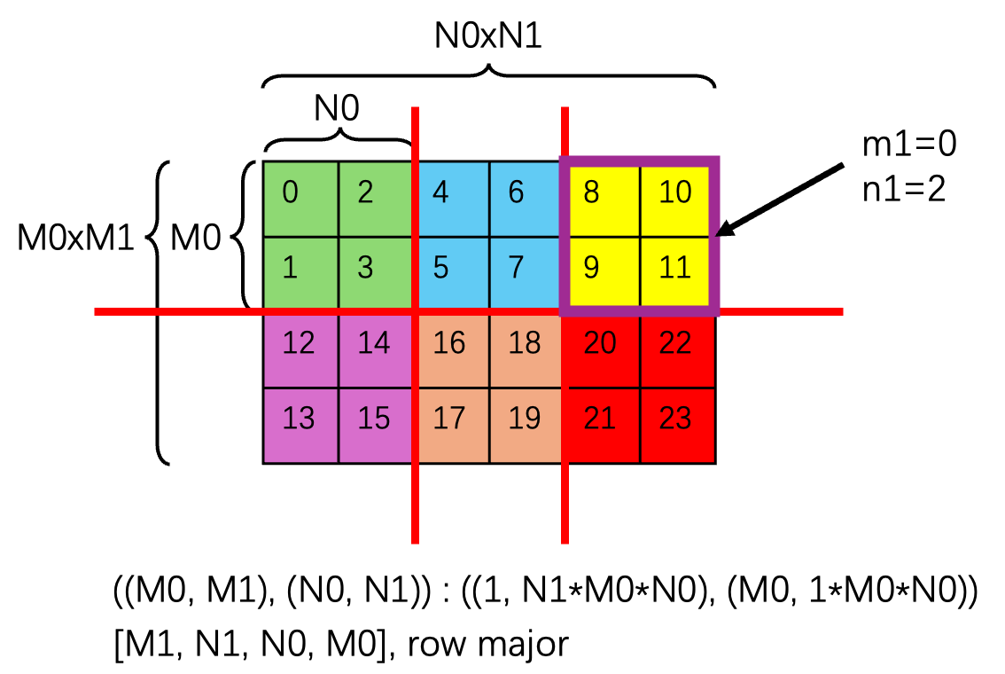
After partitioning, we end up with M1 * N1 sub-tiles (also organized in a 2d grid), with each CTA processing a sub-tile for instance. And we would want to get the sub-tile at coordinate (m1, n1). The purple box in the figure shows the sub-tile at coordinate (0, 2).

The local_tile function first does the partitioning and then does the indexing to get the 2d sub-tile (of shape (M0, N0)) at coordinate (m1, n1).

final_layout: ((M0, M1), (N0, N1)) : ((1, N1*M0*N0), (M0, 1*M0*N0))
tiler: Shape(M0, N0)
# A's layout is final_layout
local_tile(A, tiler, (m1, n1))
  = A[m1*M0 : (m1+1)*M0, n1*N0 : (n1+1)*N0]
  # and it maps to some address range in memory according to the layout of sub-tile

Two subtle things to note:

• The tiler here is not a layout but a mere tuple of shapes (i.e. (M0, N0)). This is because we are applying the partition to the two dimensions independently, they don’t interact with each other. Hence the tiler is just a tuple of shapes.
• This local_tile is not necessarily the reverse process of blocked_product. I can partition the tensor A differently from how I compose them in blocked_product, meaning M0, N0 are not necessarily the same in local_tile as in blocked_product.

6. Static vs Dynamic Integer

In CuTe, there are two types of integer: static integer (like _1{} or cute::Int<2>{}) and dynamic integer (like 3). Static integer is a compile time constant and dynamic integer is a runtime variable. The more the compile time constant, the better the compiler can reason about the code and optimize it.

Normally dynamic integer is interchangeable with static integer, with two “exceptions”:

1. Use static integers whenever possible, it is an optimization and enables other portions of code to analyze and prove their sections better. For example, the entire TMA descriptor, partitioning, certain TMA invariants due to arch, etc. can only takes certain shape of tensor tile. So it’s good to have those shape to be static/compile tile so compiler can reason about whether it can be implemented on the target arch or not. MMA is similar.
2. Rule of thumb: RMEM/SMEM/TMEM is always a static layout.

7. Summary

In this blog, we covered the basics of CuTe layout and some common operations on CuTe tensor:

• A layout consists of Shape and Stride.
• Layout is a mapping between natural coordinate and physical index in memory.
• A layout can be potentially coalesced/flattened.
• Blocked product stacks a tensor along multiple dimensions.
• Local tile is a way to partition a tensor into smaller sub-tiles.
• Static integer is a compile time constant and dynamic integer is a runtime variable.

We will explore more advanced topics such as composition, TV layout, swizzle, etc. in future blogs.

8. Additional References

• CuTe doc 01_layout
• CuTe doc 02_layout_algebra
• CuTe doc 03_tensor
• Cris’s GPU mode lecture
• Reed’s CuTe layout
• Reed’s CuTe layout algebra
• Reed’s CuTe tensor